Experiment to Produce A Spinning Electromagnetic Field
in a Cylindrical Cavity
Mode and Frequency
Used
On
this page are details of the method used and the
results obtained when carrying out the experiment to produce a spinning
field.
Also described are the problems encountered, so if you wish to carry
out
similar work I hope this information will help avoid some of the
potential
difficulties. The cavity used was chosen to be resonant in the 70cm
amateur
radio band which covers 430-440MHz and for which a transmitting license
was
available. The cavity was of cylindrical form as this was easier to
construct
than a sphere and was intended to be resonant at 435MHz in the centre
of the
band. It was decided to use a TM mode, so the lowest frequency spinning
mode
(TM110) was selected as this allowed the physically smallest size of
cavity to
be constructed. If a TE mode were used TE111 would be even smaller and
have
fewer possible interfering modes although the required measuring probe
positions would be different from those described here. The resonant
frequency
of the TM110 mode is independent of the cavity height so the diameter
can be
chosen solely for resonance at the desired frequency and works out to
84.06 cm
diameter. (See Tables of Cylindrical Cavity
Resonant Modes
for the formula used). As the resonant frequency of many of the other
modes
also depends on the cavity height it is important to choose a height
which does
not bring another resonance near to the desired one as this would make
setting
up extremely difficult. The resonant frequencies of the other modes for
the
cavity used are also shown in the Tables of
Cylindrical
Cavity Resonant Modes. Mode charts are available which show
graphically all
the resonant frequencies of a cavity and these are ideal for a rapid
frequency
selection if a different frequency is to be used. A typical Mode Chart
is shown
in Fig 30 below:-
In
this case a height of 50 cm was chosen as this
gives a ratio of diameter to height of around 1.68 ( ![]() = 2.82
) and is clear of other modes as shown by the “X”in
the above
chart.
= 2.82
) and is clear of other modes as shown by the “X”in
the above
chart.
Cavity Construction
The
cavity was fabricated from 18 s.w.g. half hard
copper sheet. The maximum length sheet available was 8ft (2.44metres)
which
meant that in order to give the required 2.64 metre circumference a
join was
necessary. For this a butt joint was used with an exterior 18 s.w.g.
backing
strip just 1.3 cm wide added for strength. It was decided to braze the
cavity
using high silver content brazing alloy. This was done in order to give
minimum
cavity losses and maximum Q. Before brazing the cylinder joints were
bolted together
and end plates temporarily held in place so that a check of the
resonant
frequency could be made. It appeared that the frequency was about
2.5MHz too
low so 1.6 cm was removed from the circumference to bring the frequency
back to
435 MHz. It was subsequently realized that it was the poor bolted
joints that
had caused the frequency reduction and it would have been better to
have
constructed the cavity to the exact calculated size. Fortunately even
with the
reduced diameter of 83.4 cm the cavity was still resonant within the 70
cm band
at just under 438MHz.
At
the required brazing temperature of 6500 C,
copper of this thickness goes very pliable and will not hold its shape
when
heated. As the gap for a brazed joint must be kept between say .02 -
.15 mm it
was necessary to rivet the joints at least every 5 cm using copper
rivets. The
circular cavity end plate was annealed and given a 1cm flange by
bending the
edges around a circular wooden former. The end plate was riveted in the
cavity
prior to brazing. After brazing it was necessary press the wooden
former
through the cylinder to maintain the cavity’s circularity. For anyone
wishing
to construct a similar size cavity I would suggest soft soldering as
this could
be done using temporary clamps instead of rivets as the soldering
temperature
is lower and the joint gaps are not so critical. The end plates could
be left
flat and soldered straight onto the cylinder ends without the need for
a flange
as the copper would distort much less. Also the copper would not loose
its
hardness at soft solder temperature which would help keep it circular.
To keep
the Q high just keep the joints as tight as possible and remove any
surplus
soft solder from inside the cavity.
Despite
having gone to such lengths to get maximum Q
it was finally decided to only braze the bottom cylinder end plate and
at the
other end a flat copper plate was just placed in position on top of the
cavity.
To make better contact it was weighted down all around the edges with a
total
of 50 kilo in weight. The loose end plate was initially used in order
to
maintain access to the cavity for fitting probes and as it did not give
any
major problems it was then left like that (so much for the high Q
construction!!). The theoretical Q for a cavity of this size is about
50,000
and a loaded Q of 20,000 was actually measured which is adequate for
this
particular experiment.
Measuring Equipment
Initially
the cavity was energized in the conventional
stationary mode. A Yaesu FT-100 transceiver was used which provided a
12 watt
radio frequency (r.f.) power source of high frequency stability and
with a
built in digital frequency readout. This source fed a small 4.5 cm
diameter
copper wire loop projecting into the cavity half way up the side.
The r.f. was fed through the cavity wall using a 50 ohm BNC
socket onto
which the loop was directly connected. By not quite fully tightening
the BNC
socket it was possible to rotate it and the loop from outside the
cavity. This
provided a very useful means of matching the loop impedance to the r.f.
source
as the effective area of the loop is the area that is normal to the
magnetic
field and the loop impedance is proportional to the area of the loop
squared.
For the modes used in these tests the maximum loop impedance is with it
positioned vertically and as it is turned to the horizontal the
impedance falls
to a low value.
For
the TM110 mode the maximum value of electric field
occurs at a distance of half the cavity radius away from the cavity
centre
axis. A ring of probes was therefore placed in the top cylinder end
plate on a
circle about the cavity centre (the circle being the same diameter as
the
cavity radius). The probes were positioned at 45 degree intervals
around the
circle. Each probe comprised a 3 cm length of copper wire connected to
a BNC
socket which provided the feed through the cavity top end plate. The
voltage on
the probes was measured using a Tektronix 2445A, 150MHz oscilloscope.
Unfortunately a higher bandwidth oscilloscope was not available but
tests showed
that although both channels suffered a 10 times reduction in
sensitivity at
440MHz, deflection was linear provided 60% deflection was not exceeded.
The
phase shift difference was within 0.18nSec and constant and unaffected
by
changing input voltage amplitude within this range. So, although not
ideal,
this instrument was adequate for the measurements to be made provided
it was
operated within the voltage limitations and the constant phase error
allowed
for. This instrument did have the advantage of having four channels.
Two of
these were of limited sensitivity and had different calibrations from
the main
channels at 440 MHz so they were not used for measurement. However,
they were
still useful for monitoring the voltage on extra probes which assisted
in initially
setting up the rotating field.
It
was found that use of the standard x10
oscilloscope probes was not possible due to signal pick up which gave
totally
unreliable readings. Instead a number of small metal boxes, each fitted
with a
BNC input plug output socket were made. An 82kohm resistor was fitted
in each
box, connected between input and output, to reduce the oscilloscope
loading. It
was found that fitting one of these isolation boxes to a cavity probe
significantly detuned the cavity but fortunately connecting the
oscilloscope to
an isolation box output did not further affect the cavity. Because of
this
eight isolation boxes were made and one connected to each cavity probe.
These
boxes should be identical and low tolerance, matched value, carbon
resistors
used. Connection from these isolation boxes to the scope was with about
a metre
of 50 ohm RG58C/U coax cable fitted with BNC connectors. Four coax
cables were
used and all cables were initially made the same length. The cables and
isolation boxes were numbered and a particular cable and isolation box
was used
only with an assigned oscilloscope channel. The lengths of the cables
were then
adjusted slightly so that all oscilloscope channels gave identical
phase
readings. Measurements could then be made on a probe by swapping its
isolation
box for one with a monitoring oscilloscope channel attached and this
would have
a negligible effect on the cavity tuning. Using screened connections
and leads
throughout in this arrangement gave fairly stable and repeatable
voltage and
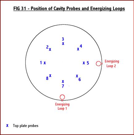
phase readings. The numbering used for the cavity probes and
energizing
loops is shown in a plan view of the top of the cylindrical cavity in
Fig 31
below. This also shows the second energizing loop which was used for
the later
spinning field tests:-
Tuning The Cavity (Conventional Mode)
To
tune the cavity the r.f. source frequency was
adjusted to give maximum oscilloscope deflection with the oscilloscope
connected via an isolation box to the cavity end plate probe number
three,
positioned opposite to the input loop. Only input loop 1 was fitted for
these
experiments and it was turned for best matching of the 50 ohm r.f.
source to
the cavity. This was determined by measuring the standing wave ratio
(SWR)
between the source and the loop using a cheap commercial SWR bridge. It
is
necessary to retune the r.f. frequency for maximum oscilloscope
deflection each
time the orientation of the loop is altered as turning the loop even
slightly
detunes the cavity. Best match was an SWR of about 2.0 and usually
occurred
with the loop turned about 20 degrees from the vertical for the 4.5 cm
diameter
loop. From theory the loop should have a low inductive reactance and
that is
why a 1.0 SWR is not obtained. It was found that if the r.f. source was
tuned
slightly away from peak oscilloscope deflection then a 1.0 SWR could be
obtained. In this condition the cavity is being tuned off resonance and
the
cavity reactance produced as a result of this is tuning out the loop
reactance.
However, a 2.0 SWR was perfectly adequate and was considered preferable
to
having the cavity detuned. Because of this most tests were carried out
with a
reduced power of only 2.5 watts in order to protect the source from the
high
r.f. voltages which can arise with a raised SWR. This still gave
sufficient
signal for measurement and also protects from the high SWR which
results if the
cavity is further mistuned. It would be possible to get a lower SWR by
using a
matching circuit but the additional complication was again considered
unnecessary at these power levels.
For
a small coil the magnetic field is a maximum
passing through the centre of the loop. However, there is also a
magnetic field
produce at right angles to this off the sides of the loop. As the size
of the
loop is increased the proportion of field off the side increases
relative to
the field through the centre. These two loop fields energize the same
cavity
mode (ie TM110 in this case) but the two modes are at right angles to
each
other. If the cavity is not exactly circular the two modes will have
slightly
different resonant frequencies and the two resonant peaks in the cavity
probe
voltages may be observed. The main mode being measured here has a
maximum
electric field adjacent to the loop (i.e. probe 7) and also 180 degrees
around
the cavity diameter from this (i.e. probe 3). This can be checked by
measuring
the voltage on all the cavity end plate probes. In all tests the peak
to peak
voltage was measured on the scope and is what has been used in the
typical
results shown below:-
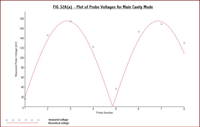
Fig
32A(a) also shows the theoretical shape of the
voltage readings it would be expected to obtain at the cavity probes.
It has
the shape of an |A sin(ф-ε)| curve where ф
is the phase angle around the cavity measured from the
point of minimum field and the amplitude (A) and phase error (ε) have
been
selected to best fit the experimental results. Each probe is spaced 45
degrees
so the phase error can be obtained from the zero of the best match
theoretical
curve, which is at 4.85 instead of 5.00, so the error is 45 x (5.00 –
4.85) =
6.75 degrees. It could be due to misalignment between the end plate
probes and
the energizing loop. However it is most likely due to a small voltage
being
present from the field off the end of the loop which is adding to the
main
field and altering the null position. Apart from this the measured
voltages are
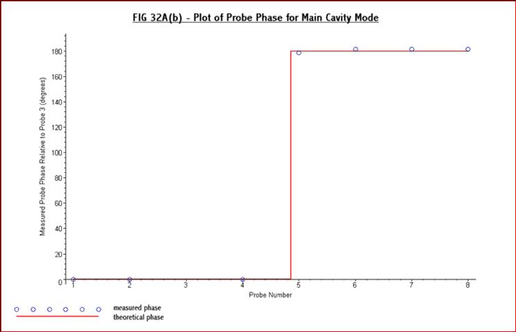
in reasonable agreement with the theoretical values. The frequency was
438.39870MHz. Fig 32A(b) below is the plot of the phase measured
between
probe 3 and each of the other probes. This was obtained by measuring
the time
difference in reaching the peak voltage and this is also as expected
for a
TM110 cavity mode:-
If
the cavity is tuned to the second mode which is
being energized by the field off the end of the loop this will be when
the
field at the probes 90 degrees from the loop (probes 1and 5) is a
maximum. In
this case it was at a frequency of 437.3621 MHz, just over 1 MHz below
the main
mode. Depending on the shape of the cavity it could easily have been up
to 1
MHz or more above. A typical set of peak to peak probe voltages and
phase
readings is:-

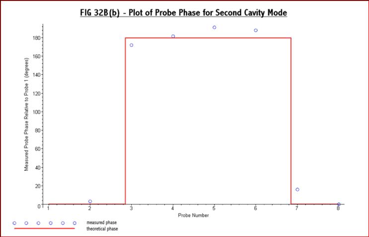
The
theoretical voltage curve is now of |A'
sin(ф-90-ε)|. Despite the phase measurements not fitting the
theoretical curve so well the readings clearly confirm that the
theoretical
TM110 mode is still being energized and that it is at right angles to
the
previous main mode. In this case probe 1 was used as reference as probe
3 has a
low voltage so it would be more difficult to take accurate phase
readings to
this probe without switching ranges on the oscilloscope which was not
permissible. The SWR for this mode was 5.5 and was with the coil
vertical which
indicates that there is a poorer impedance match. However, even so, the
maximum
cavity probe voltage was almost identical to that obtained for the main
mode.
It
was found that both modes went to a minimum when
the energizing loop was rotated to the horizontal position. This
provided a
useful means of confirming the loop position when the cavity was
completely
assembled.
How
to Produce the Spinning Mode in the Cavity
The
standard method of producing a rotating field is
to use two energizing loops spaced 90 degrees apart around the
circumference
and fed with signals time displaced 90 degrees. This is similar to the
way a
two phase motor produces a rotating field. It is just as applicable at
r.f.
frequencies and is the best method found to produce a purely spinning
field.
The voltage plots in Fig 32A and 32B for the single loop stationary
modes
confirm that the field in the ф direction is sinusoidally distributed
and
it is also known that it is varying in amplitude sinusoidally. We can
show
mathematically that a spinning field is produced by writing the field
from the
single loop as:-
E1 = F.![]()
Where
F is a function representing the field
distribution in the radial and z (height) directions. NB. The
expressions used
for the phases are just representative, no attempt has been made to
match them
to actual loop positions used.
If
there is another loop 90 degrees apart around the
circumference and the current is 90 degrees phase shifted then the
field from
this loop will be:-
E2 = F.![]()
The
combined field with the two loops energized will
be the sum of these two fields:-
Et = E1 + E2 = F(![]() +
+![]() )
)
Using
the standard trig relationships:-
2cosAcosB
= cos(A+B) +cos(A-B)
and
2sinAsinB=cos(A-B)-cos(A+B)
This
gives:-
Et = ![]() (cos(ф-ωt)
–cos( ф+ ωt) + cos( ф+ ωt) + cos(ф-ωt))
(cos(ф-ωt)
–cos( ф+ ωt) + cos( ф+ ωt) + cos(ф-ωt))
= F
cos(ф-ωt)
(1)
In
some respects this is just a different way of
writing the addition of two stationary fields but it also represents a
completely new field system which is physically spinning in the +ф
direction. The reality of the spinning field in the similar two phase
motor
case is apparent from the rotational speed and torque developed by the
motor
and is just as real, although not so obvious, in this r.f. field.
The
simplest way to produce the required current phase
difference is by feeding the two loops in parallel and using a quarter
wavelength longer feed line to one of the probes. Ideally, if the loop
impedance is 50 ohm then connecting them in parallel would present the
r.f.
source with a 25 ohm impedance. However, a quarter wavelength of 75 ohm
line
will convert a 50 ohm impedance to 100ohms so this was used in each
loop feed
line to convert the loop impedance to 100 ohm so the parallel impedance
would
be 50 ohm. A diagram of the phasing line used is shown in Fig 33 below:-
The
phase delay produced by a length of line does not
normally just depend on its length as the reactive impedance of the
load also
affects it considerably. Fortunately for lines which are exact
multiples of a
quarter wavelength, such as are being used here, the phase delay is
independent
of reactive impedance. If the two loops have the same reactance the
extra
quarter wavelength in the loop 2 line will convert it’s reactance
from
inductive to capacitive so when the two are connected in parallel there
will be
a tendency for the reactances to cancel, although not normally exactly.
However, this is the ideal case and one problem is mutual inductance
between
the loops and this will be opposite for each loop as the voltage from
one loop
will be in phase by the time it reaches the other but the voltage
from
the other loop will be in antiphase at the other. It was thought
that
this might be a problem and in practice the best spinning field was
obtained by
tilting the two loops to different angles so the above theoretical
perfectly
matched condition was not used. However, using this phase delay line it
was
found possible in practice to adjust the currents in the loops to
obtain a
spinning field provided an SWR of about 2 was acceptable at the r.f.
source,
which it was.
A
quarter wavelength in free space is about 70/4 =
17.5 cm long. This is not the length required for a quarter wavelength
of
coaxial cable as the wave in the cable only travels at about 0.65 of
the free
space velocity. This is known as the velocity factor and varies
depending on
the cable construction. A quarter wavelength of coax is therefore
approximately 17.5x0.65 = 11.4 cm long. Experimental methods to obtain
an exact
electrical length of coax cable rely on the fact that an open circuit
quarter
wavelength of line (also ¾, 1¼…etc wavelength) will appear to be a
short
circuit if the impedance is measured at one end. Conversely a short
circuited
half wavelength (also 1, 1½, 2…etc wavelength) of cable will appear to
be open
circuit if the impedance is measured at the opposite end to the short.
If you
have an r.f. impedance bridge you can measure the cable impedance
directly. If
not there are various simple techniques available which make use of
these
characteristics. The main error is due to additional impedance caused
by the
measuring system and cable terminations used. The method adopted here
was with
the r.f. source, set to the resonant frequency of the cavity, used to
apply an
r.f. voltage to the cable under test. The test length of cable was
energized
through a resistor network so that when the cable was a quarter
wavelength long
the voltage across it, which was monitored using the oscilloscope,
would be a
minimum. The circuit used is illustrated below. The two resistors
ensure the
source always feeds into a reasonable SWR load:-
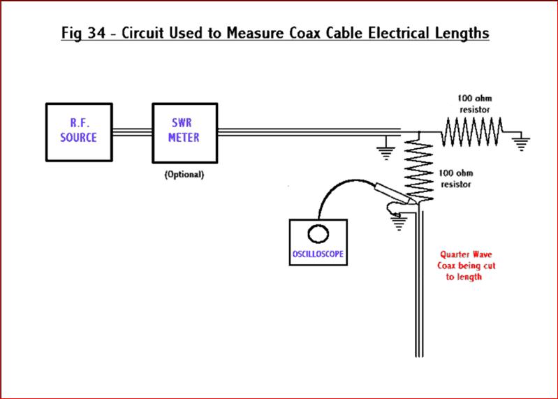
The
earths were connected to a small copper plate and
made as short as possible and the resistors were carbon. The coax line
under
test is cut, removing about 3mm at a time and the voltage on the scope
recorded
each time. The minimum voltage will be reached when the line is a
quarter
wavelength long. It is likely you will overshoot first time but the
required
length will now be known. The same technique can be used to find a
¾
wavelength. (and if it’s not three times the length of the quarter
wavelength
cable you have a problem with the technique!). Half wavelength could be
found
by repeating the procedure but with a short circuit on the far end of
the line.
However due to the inconvenience of fitting the short it is easiest to
just use
a cable twice as long as the measured quarter wavelength.
Tuning the Cavity for
the Spinning Mode.
To
tune the cavity the two loops are first energized
using the phasing line and the voltage on cavity probes one and three
monitored
on the oscilloscope. If the r.f. source frequency is adjusted either
side of
the calculated cavity resonant frequency it is likely that two peaks
will be
observed on the oscilloscope. These will be the main and second modes
measured
above. To bring the two resonances to the same frequency a substantial
octagonal
wooden frame was built around the cavity. This nominally touched the
cavity in
eight places around the diameter although the frame was constructed
slightly
oversize so that there was about 2mm clearance between the frame and
the cavity
at these points. The frame was fitted with four simple screw jacks each
with a
vertical load spreader bearing against the top half of the cavity
circular
sides at 45 degree intervals around the periphery. Two were on the same
axis as
the two energizing loops, one midway between them and one 45 degree
away (i.e.
adjacent cavity probes 4,5,6 and 7). The load spreaders were simple
hardwood
strips about 23x5x0.7cm, each with wooden block about 5x5x2cm attached
which
had a hole drilled through it to locate the screw of the jack. Four
notches
about 5.5x1cm each were cut in the octagonal frame to make room for the
load
spreaders. This arrangement is shown in Photographs
1, 2
and 3.
Adjusting
the circularity of the cavity with the screw
jacks allows the main and second resonant peaks to be brought to the
same
frequency. The tilt of the loops can then be adjusted until the
voltages on the
cavity top plate probes are as identical as possible and the phase
difference
between each adjacent probe is 45 degrees. This is the condition which
is
required for a spinning field to be produced. For this adjustment it
was useful
to have the two additional oscilloscope channels available which were
temporarily
connected to probes 2 and 4 to approximately confirm that the voltage
and phase
here appeared to be correct before a full set of all probe readings
were taken
using the two calibrated oscilloscope channels. To reach the correct
condition
requires repeated small adjustments to the r.f. frequency, cavity
circularity
and loop angle as the adjustments are very critical and inter-related.
Because
the cylinder top plate was not soldered in position the tuning could
also be
disturbed by a change in top plate contact resistance particularly as
the
cavity top plate probes were interchanged to take scope readings. So
after
taking a complete set of readings the initial probe readings were again
checked
and if these had changed significantly the results had to be discarded
and a
new set of readings taken. An example of typical readings obtained is
shown in
Figs 36(a) and 36(b) below:-
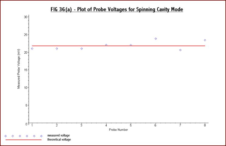
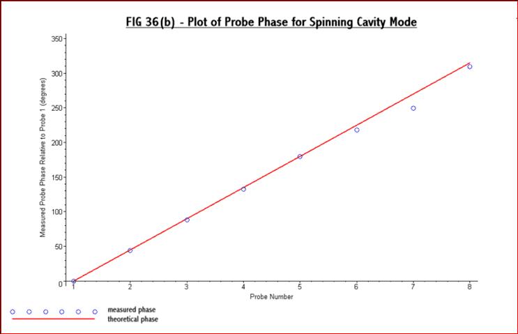
Although
the probe voltages are not quite identical
the results are in reasonable agreement with theory and indicate that a
spinning field has been produced in the cavity. This is the best
technique
found for producing a pure spinning field in the cavity.
Effect of Change in
Phase or Amplitude in the Field of an Energizing
The
affect of tuning the cavity can be analyzed
mathematically using a similar method as was done previously. If we
consider
just the main mode field and assume that these fields from the two
loops have
different amplitudes and a phase difference between them which is not
exactly
90 degrees then the equation for the field from loop 1 is:-
E1 = F.![]()
Where
F is again a function representing the field
distribution in the radial and z (height) directions.
If
the current in loop 2 is 90 degrees phase shifted
then the field from this loop will be:-
E2 = F.A.![]()
Where
A is the ratio of the field amplitudes and a
represents the phase error from the correct 90 degree phase difference.
The combined field with the two loops energized will be the sum of
these two
fields:-
Et = E1 + E2 = F(![]() +A
+A![]() )
(2)
)
(2)
The
variation of Et with time at different cavity top
plate probes (ie values of phi) can be plotted for various values of A
and a.
First assuming the phase difference is constant at 90 degrees (ie a
is zero) the effect of a change in A, the relative amplitude of the
current through one of the coils is shown in Fig 37:-
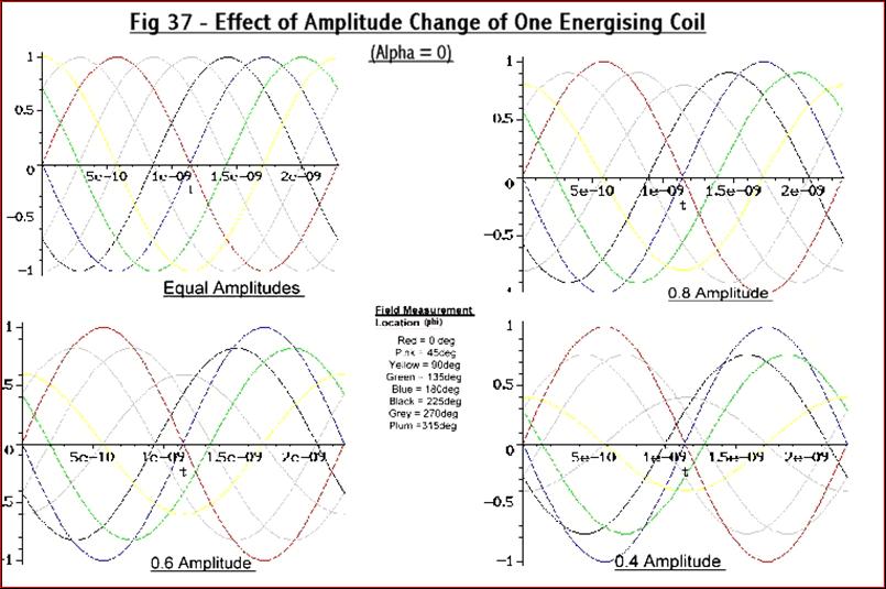
It
can be seen from these plots that with equal field
amplitudes from the two loops the voltage measured at all the top plate
cavity
probes will be the same and the phase difference measured between them
will be
the same as their physical angular separation (i.e. 45 degrees in this
case).
This is the purely spinning field which was also created experimentally
as
shown previously in Figs 36(a) and 36(b).
As
the field produced by one of the loops reduces the
voltage on the cavity probe adjacent to the loop and directly opposite
it also
reduce. The phase difference between the maximum and minimum voltage
probes
(which are either adjacent or opposite the loops) stays fixed at 90
degrees but
the phase difference between a probe at maximum voltage and a probe 45
degrees
from it reduces considerably.
If
the amplitudes are the same but the phase
difference varies from 90 degrees, by the angle alpha, then the
measured fields
will be:-
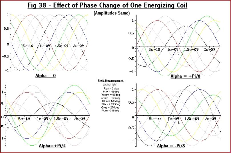
In
this case when the phase difference between the
energizing coils deviates from 90 degrees it will affect the amplitude
as well
as the phase of the voltages measured at the top plate probes.
The
above two figures show the sort of effects that
are observed when tuning the cavity for a spinning field. If just two
cavity
probes are to be observed for the initial tuning then one technique is
to use
two probes physically spaced 45 degrees apart (probes 1 and 2) and
adjust for
equal voltages and 45 degree electrical phase displacement. Then check
two
probes spaced 90 degrees apart and opposite the energizing coils
(probes 1 and
3) to check that each of the two component fields are the same
magnitude.
The
above analysis illustrates the difficulty in
obtaining a set of readings in which all probe voltages are exactly the
same
magnitude and the phase difference between them is the same as their
physical
angular separation. This would only occur if the two component fields
were
absolutely identical in amplitude and have exactly 90 degrees phase
difference.
If this condition were not exactly met then a spinning field would
still be
produced but in addition there would be a small conventional stationary
field
superimposed on it.
Obtaining a Spinning
Field With Just One
The
above explanation for obtaining a spinning field
from two loops has for simplicity assumed that each loop only produces
a main
cavity mode. In practice the loops also produce a substantial second
cavity
mode at right angles to the main one. It was observed that the optimum
spinning
field was obtained not with the two loops rotated to the same angle but
with
loop 2 almost vertical and loop 1 almost horizontal. This means that
loop 1
would have been making only a minor contribution to the total cavity
field. The
most likely reason for this is that the second cavity mode produced by
loop 2
is providing a large portion of the required field it has previously
been
assumed loop 1 main mode would produce. The spinning field is still
being produced
by two fields at right angles and with a 90 degree phase difference but
the
source of each of these two fields is not solely its associated loop.
To
test this a further experiment was done with just
loop 1 energized but the cavity circularity was adjusted to bring its
main and
second modes to the same frequency to see if a spinning field could be
produced. For a spinning field it would require the main and second
modes to be
equal amplitude. Looking at Fig 32A(a) and Fig 32B(a) it can be seen
that for
the 4.5cm diameter loop used they very nearly are. There must also be a
90
degree phase difference between them. Typical results obtained are
shown in Fig
39(a) and Fig 39(b) below:-
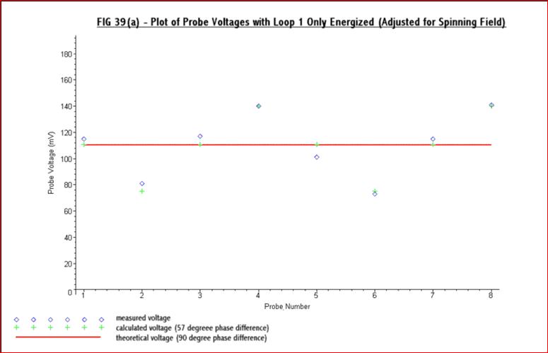
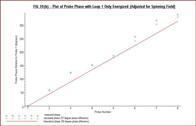
The
above figures confirm that just one loop is able
to produce a substantial spinning field. Fig 39(a) indicates that out
of a peak
probe voltage of 140mV the spinning field is just over 70mV. It
is
possible to re-plot equation 2, for the total field (i. e. Et = F(![]() +A
+A![]() )
), to give the
calculated phase difference and voltage at the probes. This has been
done on the
above figures and is shown by the green crosses for a phase error (α)
of
33 degrees. This is equivalent to a phase difference of 57 degrees
between the
main and second fields, assuming that they are the same amplitude. This
phase
error gives the best fit to the actual readings and so it is reasonable
to
assume that this is the phase error which existed when the test results
were
taken. It was found difficult to improve on this with just one loop
energized
as the only adjustment available was the circularity of the
cavity. It
does, however, illustrate the ease with which a limited amount of
spinning
field can be produced.
)
), to give the
calculated phase difference and voltage at the probes. This has been
done on the
above figures and is shown by the green crosses for a phase error (α)
of
33 degrees. This is equivalent to a phase difference of 57 degrees
between the
main and second fields, assuming that they are the same amplitude. This
phase
error gives the best fit to the actual readings and so it is reasonable
to
assume that this is the phase error which existed when the test results
were
taken. It was found difficult to improve on this with just one loop
energized
as the only adjustment available was the circularity of the
cavity. It
does, however, illustrate the ease with which a limited amount of
spinning
field can be produced.